Experiment 6: Electromagnetic Radiation Lab

Purpose:

       The purpose of this experiment is to investigate the behavior of electromagnetic radiation due to a simple antenna.

Experiment:

A piece of copper wire connected to a frequency generator acts as the transmitter.

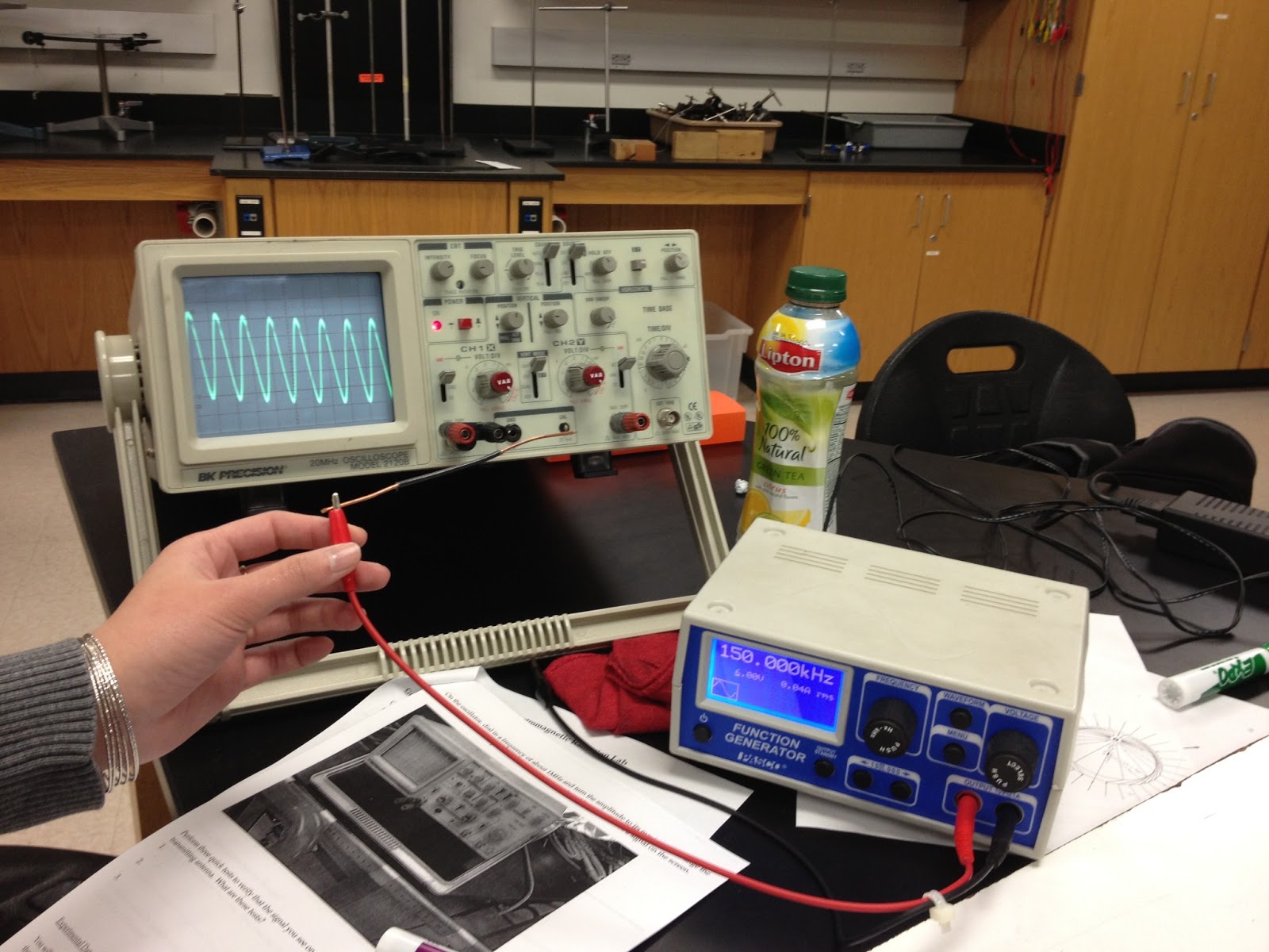
The BNC adapter is used as the receiver and is connected to an oscilloscope. The oscilloscope and receiver will detect the electromagnetic wave as shown

To verify that the signal on the oscilloscope is actually generated by the transmitting antenna, we can do the following tests:

1. Move the wire back and forth to see if there's a change in wave shown in the oscilloscope
2. Unplug the detector
3. Turn off the function generator

Data:
We are measuring the peak to peak amplitude of the received EM wave as a function of the distance from transmitter.

Distance (m)	# of divisions peak to peak	Vertical scale(mV)	Peak to peak amplitude (mV)
0 ± 0.02	3.5 ± 0.1	50	175 ± 5
0.05 ± 0.02	1.2 ± 0.1	50	60 ± 5
0.10 ± 0.02	3.2 ± 0.1	20	64 ± 5
0.15 ± 0.02	2.9 ± 0.1	20	58 ± 5
0.20 ± 0.02	2.8 ± 0.1	20	56 ± 5
0.25 ± 0.02	2.4 ± 0.1	20	48 ± 5
0.30 ± 0.02	2.2 ± 0.1	20	44 ± 5
0.35 ± 0.02	1.9 ± 0.1	20	38 ± 5
0.40 ± 0.02	2.0 ± 0.1	20	40 ± 5
0.45 ± 0.02	1.5 ± 0.1	20	30 ± 5
0.50 ± 0.02	3.8 ± 0.1	10	38 ± 5
0.55 ± 0.02	3.6 ± 0.1	10	36 ± 5

Graphs of peak to peak amplitude as a function of time
As a function of A/r + B:

As a function of A/r^2 + B:

As a function of A/r^3 + B:

The graphs above have shown that the function A/r + B best fits the data. Our results might have differ from a 1/r function because of the approximation used when calculating field near the transmitter. The near field and far field vary as two different functions.

Analysis:

Theoretical Analysis

From the calc variant, we calculated:

where:

   L = 0.1 m

   k = 9 * 10^9 N^2 * m^2 / C^2
   Q = 1.24 * 10^(-10) C
   V_0 = 40.29 mV

Therefore,

Distance (m)	Theoretical Amplitude (mV)
0.05	59.99751
0.1	51.0499
0.15	47.61179
0.2	45.82335
0.25	44.73271
0.3	43.99963
0.35	43.47352
0.4	43.07777
0.45	42.76936
0.5	42.52229
0.55	42.31994

When compared with the experimental plot

Even though there is a fluctuation in the experimental plot, we can still see that the experimental and theoretical plot has the same trend.

Uncertainty Analysis:

Voltage uncertainty:  ΔV = ± 10 mV (for a scale of 50mV)

                                       = ± 4 mV (for a scale of 20mV)
                                       = ± 2 mV (for a scale of 10mV)

Distance uncertainty: Δz = ± 0.001 m (operational error)

                                     = + 0.02 m (system error)

Total distance uncertainty: Δz_total = + 0.021 m / - 0.001 m

Using the uncertainty in distance, we can calculate the range in which the theoretical values actually lie:

Distance (m)	Voltage max (mV)	Voltage min (mV)
0.05 (+0.021/-0.001)	60.32	54.96
0.1 (+0.021/-0.001)	51.15	49.29
0.15 (+0.021/-0.001)	47.66	46.74
0.2 (+0.021/-0.001)	45.85	45.31
0.25 (+0.021/-0.001)	44.75	44.39
0.3 (+0.021/-0.001)	44.01	43.76
0.35 (+0.021/-0.001)	43.48	43.29
0.4 (+0.021/-0.001)	43.08	42.94
0.45 (+0.021/-0.001)	42.77	42.66
0.5 (+0.021/-0.001)	42.53	42.43
0.55 (+0.021/-0.001)	42.32	42.25

The uncertainty in the peak to peak voltage can be shown in the graph below

When compared with each other,

we can see that even though the experimental and theoretical graphs have the same trend, they don't actually agree within uncertainty

Discussion:
Our model assumes that the receiver is a single point and that the center of the transmitter lies on the line along the receiver. Our results are also affected by equipments around the lab area. We found that electronics, including the function generator that we use, affect the reading on the oscilloscope.